Predict Infrared Spectra

This tutorial will demonstrate how to predict IR spectra using density functional theory and compare the predicted spectrum with experimental results. All of the calculations and analysis can be performed on your laptop using a simple graphical interface.

This tutorial requires local installation of ORCA and ChimeraX (plus the SEQCROW extension to ChimeraX). Instructions for setup can be found here. All of the input, output, and analysis files for the calculations in this tutorial can be found here. The files are provided so that so that you can play around with visualization and analysis before running your own calculations.

Table of contents

1. What are these peaks?
2. Substitute Substituents in ChimeraX
3. Generate Input File and Run Calculation
4. Visualize Vibrational Modes
5. Visualize IR Spectrum

What are these peaks?

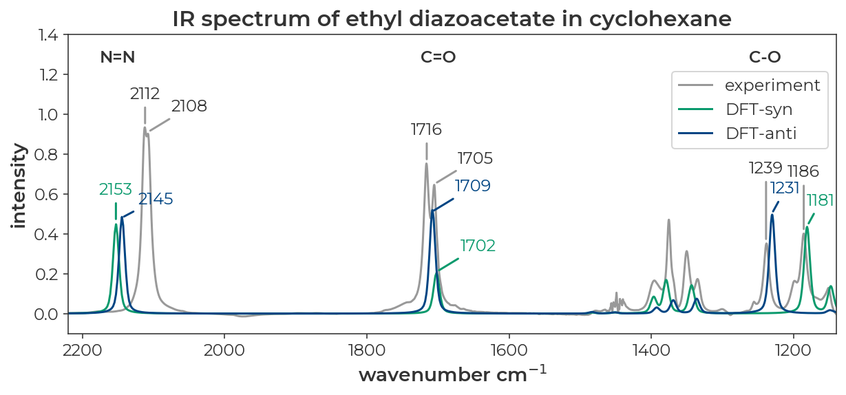
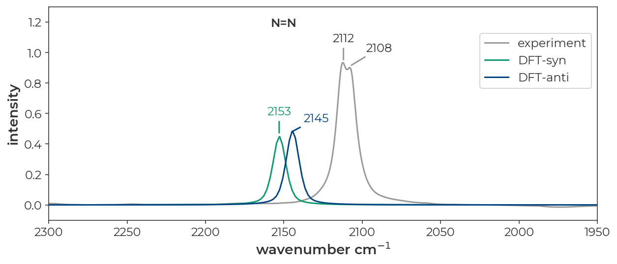
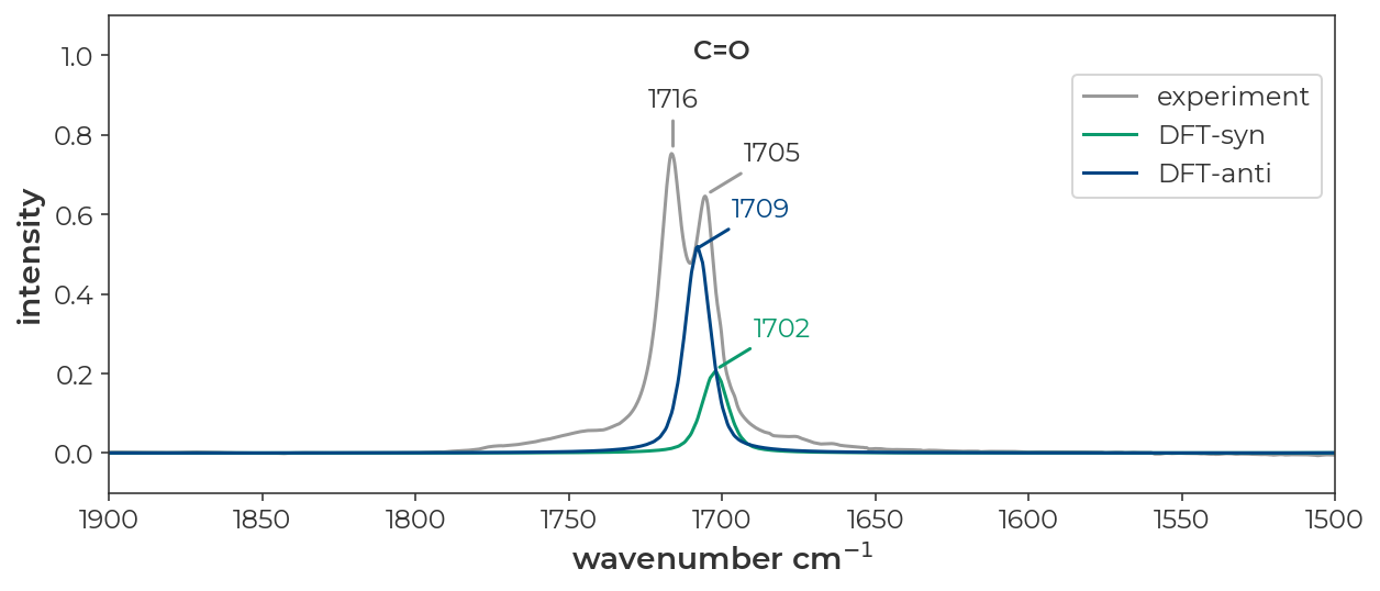
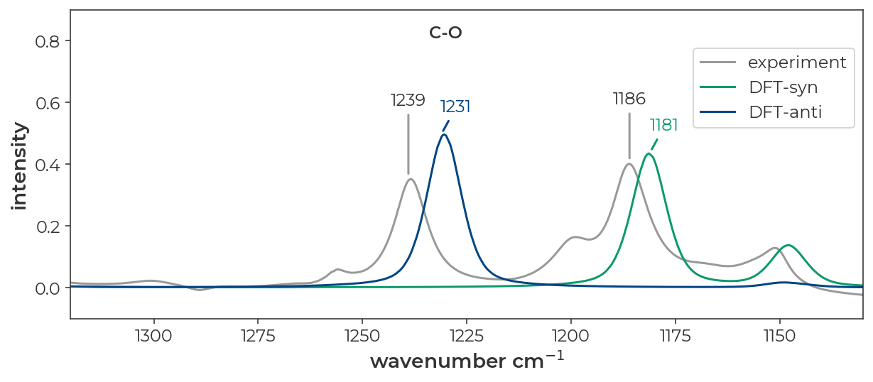
The IR spectrum of ethyl diazoacetate in cyclohexane looks like it has two distinct peaks for the N=N, C=O, and C-O stretches (JACS 2022, 9330-9343).

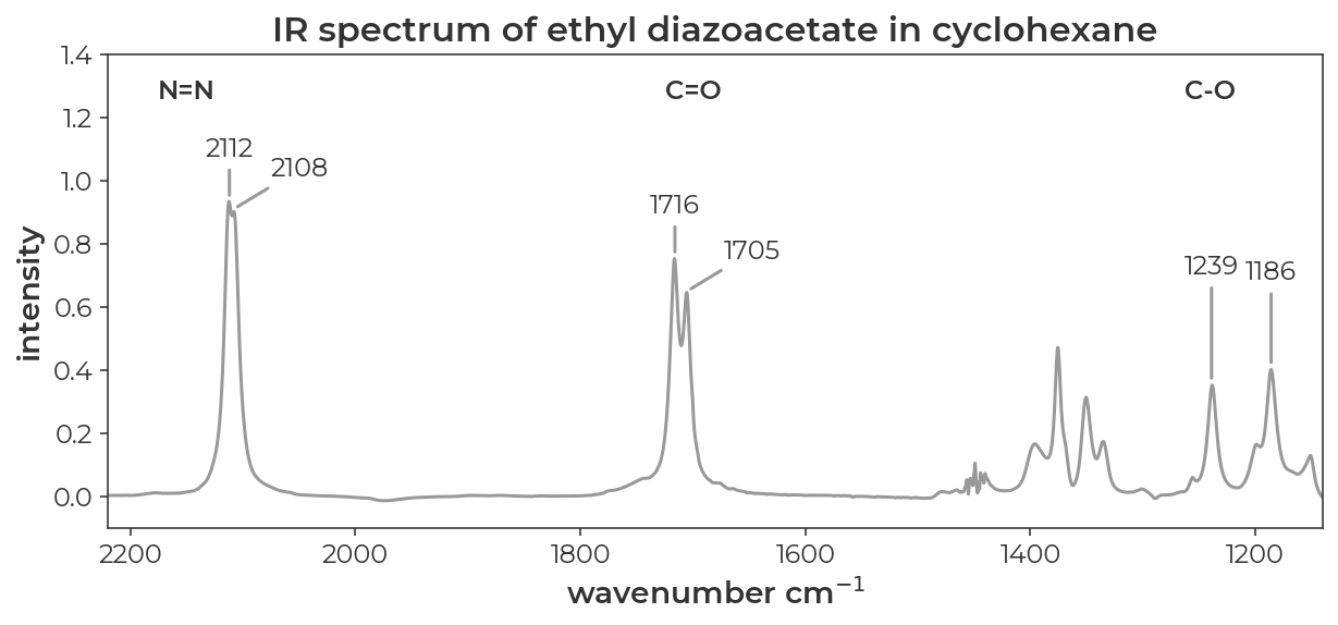
Data from SI of JACS 2022, 9330-9343

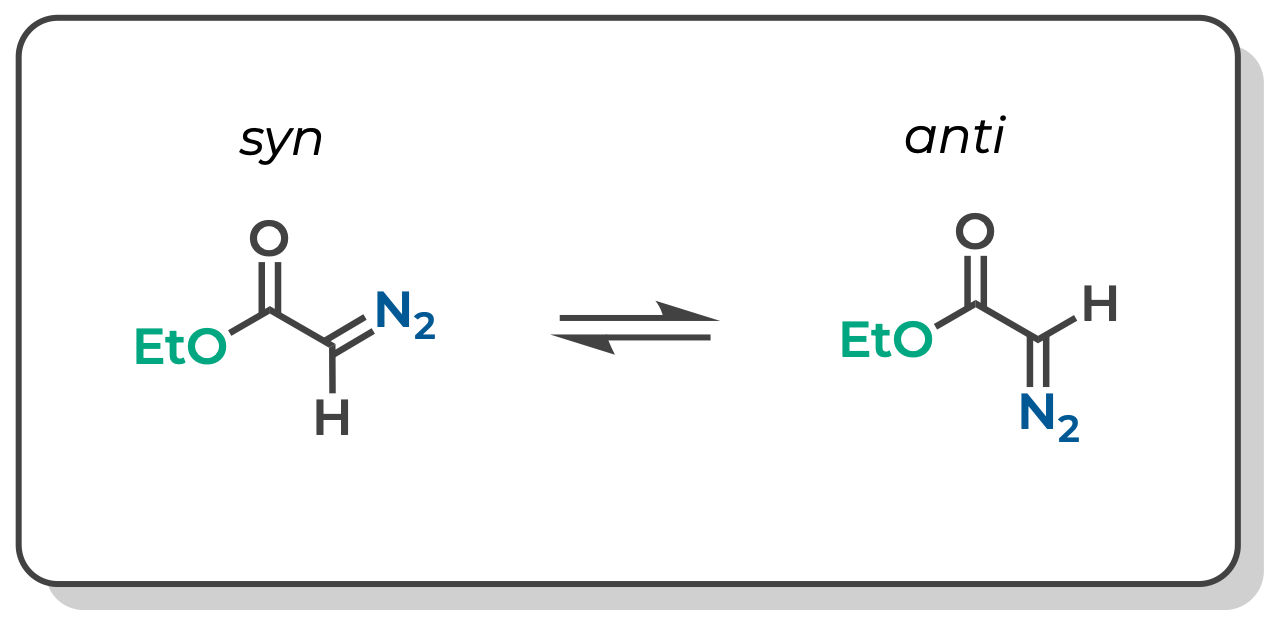
We saw in another tutorial that methyl diazoacetate is a nearly equal mixture of syn and anti conformers. If we assume that these pairs of peaks correspond to the syn and anti conformers, could we use DFT to assign which peak corresponds to which conformer?

Substitute Substituents in ChimeraX

We already have an optimized structure of methyl diazoacetate from a prior tutorial. We can open this structure in ChimeraX and modify the methyl substituent to generate an initial guess for the input geometry of ethyl diazoacetate. Tools > structure editing > change substituent. In the windown for ‘substituent name:’ add ‘Me’. In the GUI window, select ‘More Right Mouse’ and ‘Substitute’. Then right click on one of the hydrogens on the methyl group of methyl diazoacetate to substitute the H for Me. The added substituent is shown in space filling mode to give a sense for potential clashes.

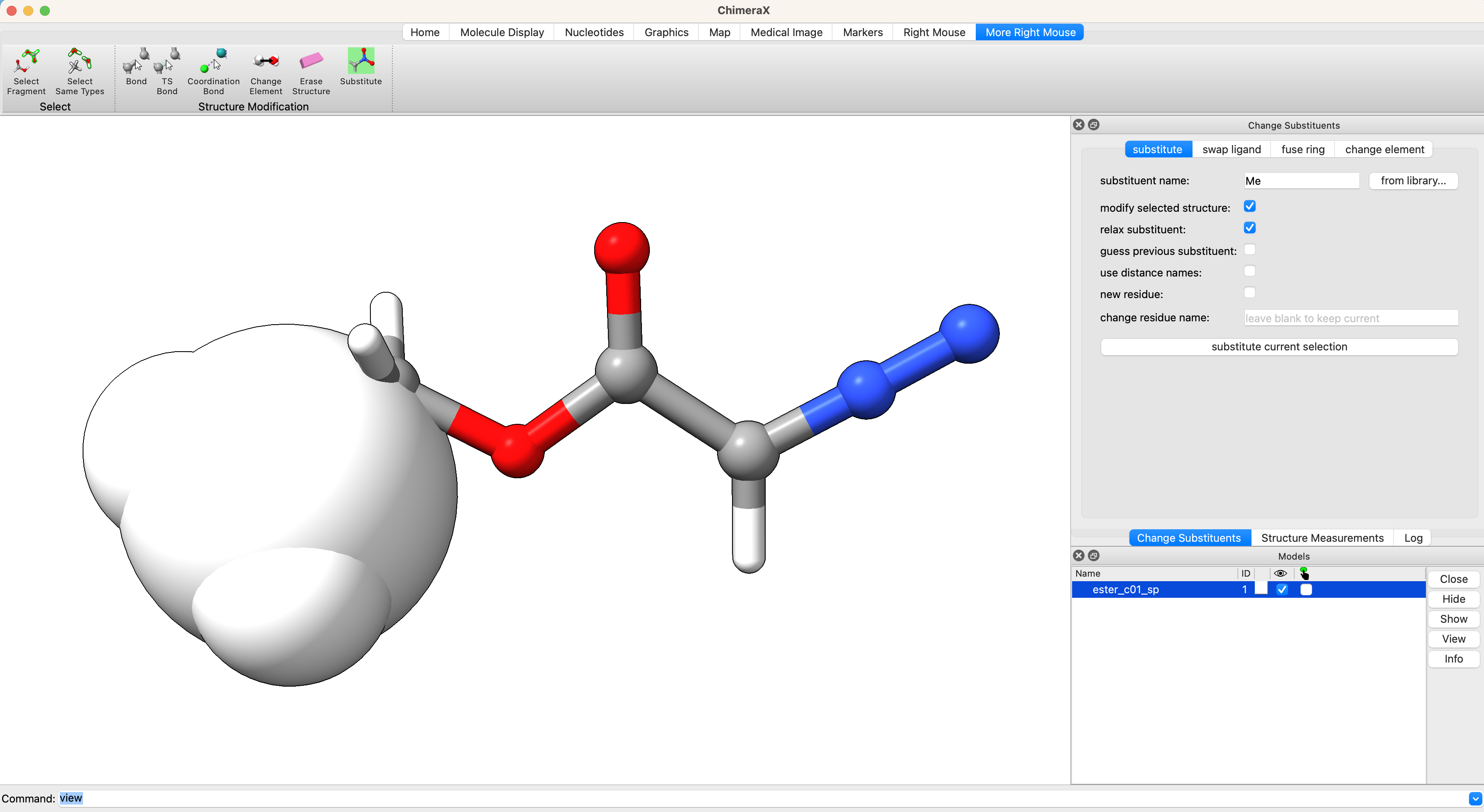
Follow the same procedure to generate the input structure of the anti conformer.

Generate Input File and Run Calculation

With the updated geometry, we will generate and submit the job in the same way we did in the prior tutorial. The only significant change to the method is that we will use cyclohexane (the solvent used for the experimental spectrum) as the implicit solvent model and we will use 6-31G* as the basis set because vibrational scaling factors are readily available.

! B3LYP tightscf Freq Opt 6-31G* CPCM(CycloHexane)
%pal
    nprocs 1
end
%MaxCore 1000
%freq
    Temp    298.15
end

*xyz 0 1
C     0.917852  -0.637477  -0.212483
C    -0.307682   0.128522  -0.016164
N     2.049677   0.016640  -0.238808
O    -1.373434  -0.692560  -0.012876
O    -0.375873   1.334518   0.125684
C    -2.649232  -0.071566   0.170809
N     3.020133   0.598093  -0.258681
H     0.960640  -1.719095  -0.339346
H    -2.698332   0.437846   1.145350
H    -2.844281   0.663409  -0.624848
C    -3.674601  -1.192126   0.112821
H    -3.650137  -1.676924  -0.886065
H    -4.692047  -0.784480   0.291735
H    -3.448628  -1.953203   0.889415
*

We can submit this job from the ChimeraX GUI in the same way we did in the prior tutorial. The optimization and frequency calculation took just under 8 minutes on my computer. Perform the same geometry optimization and frequency calculation for the anti isomer. You can find all of my input and ouptut files here (download diazo-ir-in-out-files.zip).

Visualize Vibrational Modes

Once the optimization is complete, we can visualize the normal modes of interest from the dropdown menu Tools > Quantum Chemistry > Visualize Normal Modes.

Visualize IR Spectrum

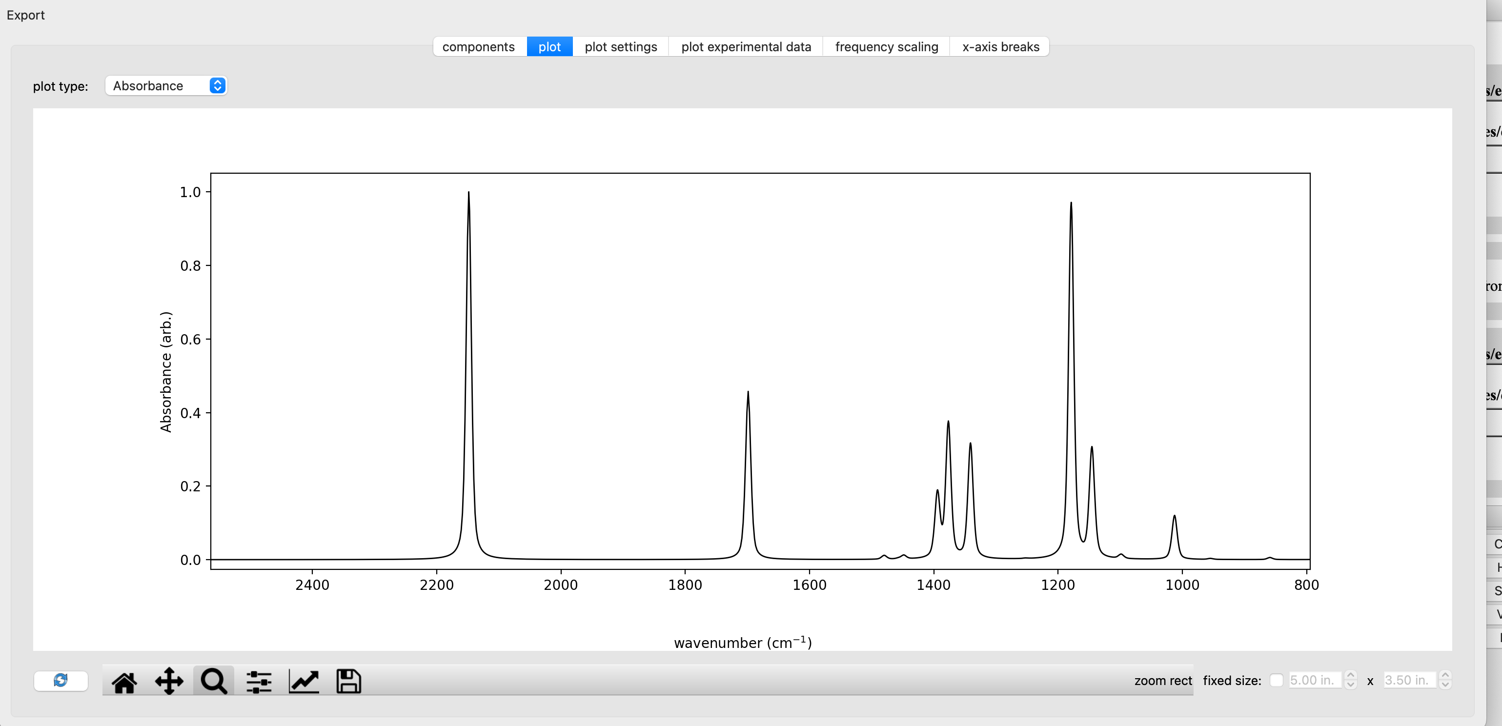
From a computational output file containing a frequency calculation, one can visualize a modeled IR spectrum in ChimeraX+SEQCROW. With eda_syn.out open in ChimeraX, go to Tools > Quantum Chemistry > IR spectrum. The spectrum can be scaled in the frequency scaling tab. Here we use scalimg factors for B3LYP/6-31G(d) as the method/basis set. The scaled computed spectrum of the syn conformer of ethyl diazoacetate is shown below.

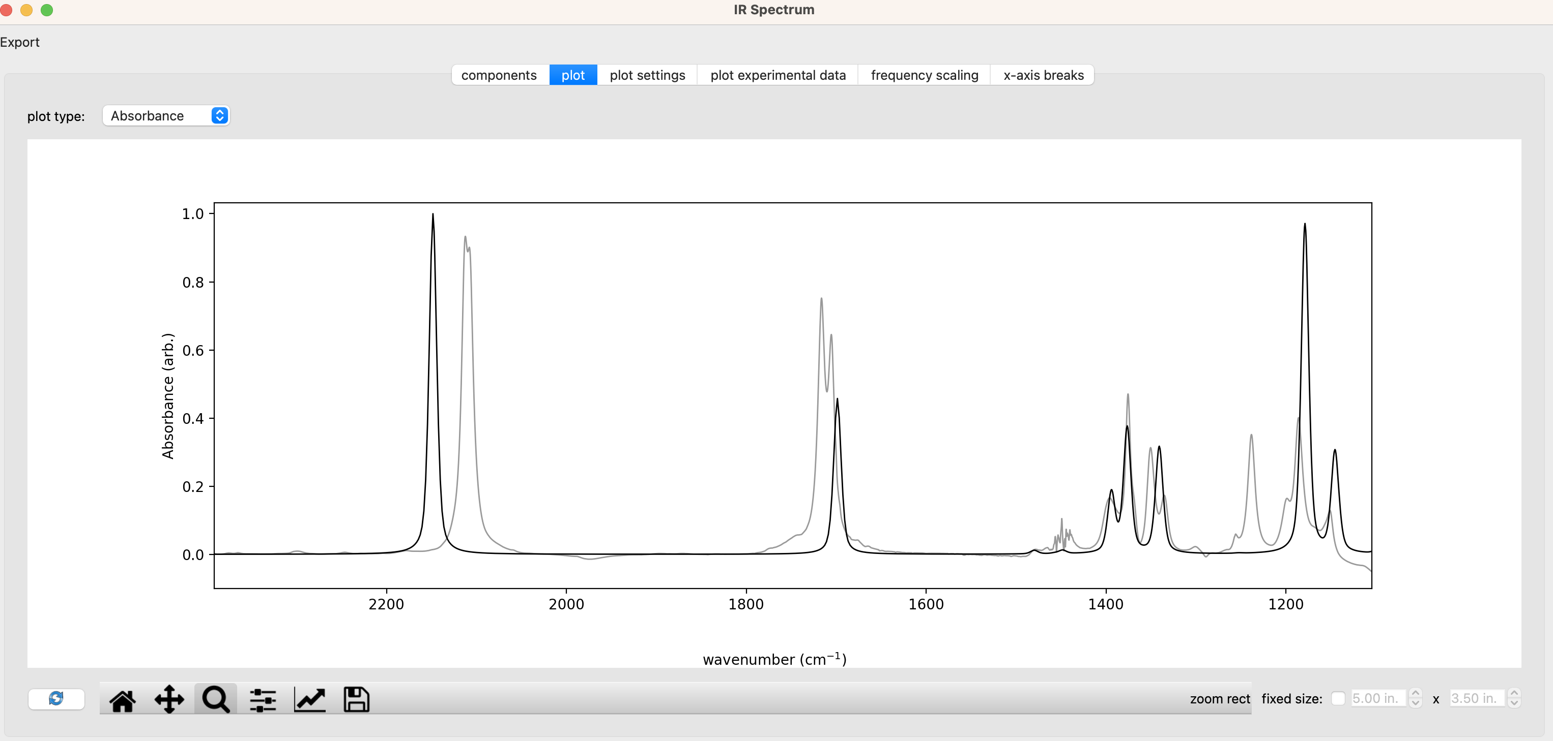
We can overlay the calculated and experimental spectrum in the ‘plot experimental data’ tab. A CSV of the experimental spectrum reported in JACS 2022, 9330-9343 can be found here. Be sure to set ‘skip first lines:’ to ‘1’ to account for the fact that the first line includes column titles rather than data. The overlaid spectrum is shown below with the experimental spectrum in grey and the computed spectrum for syn-EDA in black.

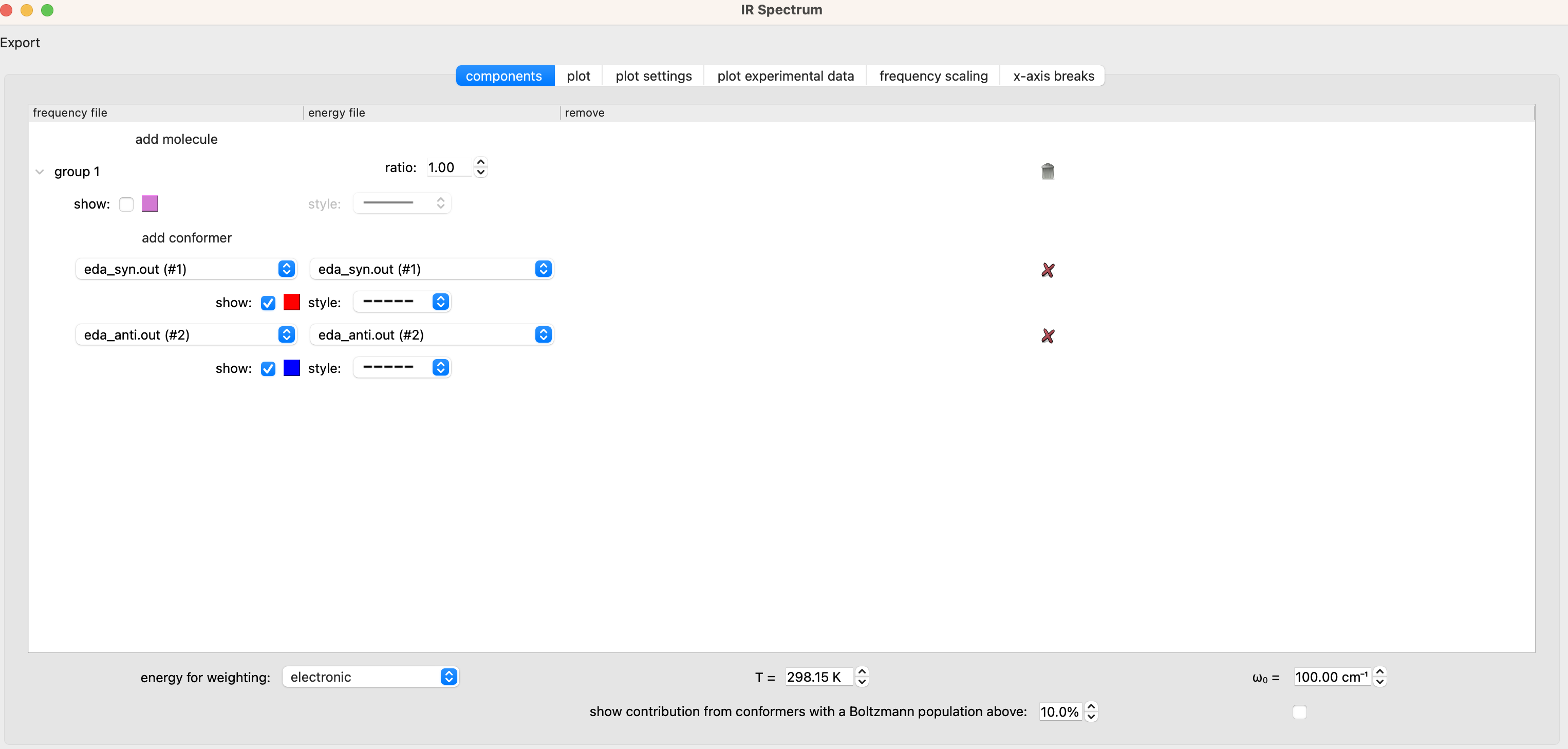
We can then compare the IR spectra of the syn and anti conformers to the experimental spectrum. With both the syn and anti output files open in chimeraX, go to the IR Spectrum window, select the components tab and select ‘add conformer’. Set the new conformer to eda_anti.out for both the frequency file and energy file.

The resulting spectrum is plotted below with the experimental spectrum in grey, the computed syn spectrum in red, the computed anti spectrum in, and the sum of the two computed spectra in black. I’ve used the ‘x-axis breaks’ tab to zoom in on the regions of interest. These data can be exported to a CSV file with the ‘export’ button in the upper left corner of the ‘IR spectrum window’. The resulting CSV can be used for plotting in excel or other plotting software.

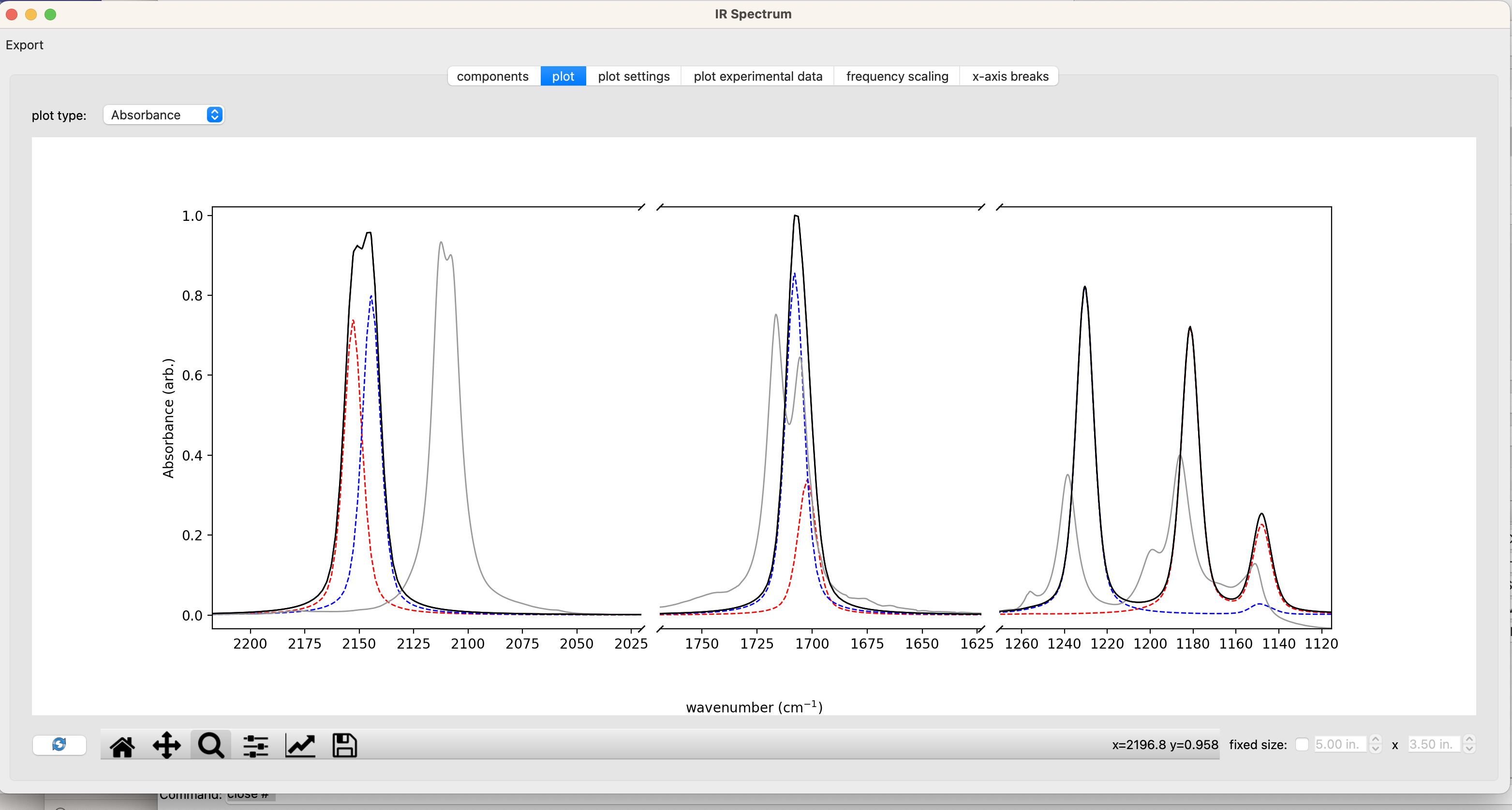
Below, I’ve replotted the data in a JupyterNotebook. The overall message is that DFT does a good job of recapitulating the absolute stretching frequencies of both isomers and predicts differences in the spectra of the syn and anti isomers that line up nicely with the pairs of peaks observed in the experimental spectrum.